Viewers we described formatting of cells
and Excel worksheets of Microsoft Excel in previous articles. During which we
had discussed formats for digits, dates, text and special codes values. New we
will require revised formats after inserting new data in excel datasheet having
different digits, dates and text etc. So, we will again change our format.
Suppose we have to set the eldest student in our class. Then we will analyze
birthdate of every student. But Microsoft Excel facilitates to highlight eldest
student of the class. We can set all types of these options through setting
conditional formatting in excel. Following is the method to apply conditional
formatting in MS Excel:-
How to Apply Conditional Formatting in
Excel
Conditional formatting assists to analyze
data as answer specified in mind. For instance, we have to collect rupees
259600 from students on account of monthly fees. If we may set it according to
our target, but it is received lesser than the specified amount then it will be
highlighted as per given settings. We can apply conditional formatting on a
cell, table or pivot table as per our need. We can set conditional format in
numbers, icons, colors and other format changes based on conditions. If the set
conditions are true then prescribed formatting will be shown as set by us
otherwise it will show other formats. We will describe to apply conditional formatting
in succeeding paragraphs.
Suppose we have not to receive monthly
fees from the students of Class 6th from 1500, and then we have to set the
conditional formatting if fees amount is less than 1500. We will follow under
mentioned method to apply this condition.
Select whole column H upto last row of
student fees, then click on conditional formatting. Options showing tables
formats, icons format etc will be shown and where you see at end also “New Rules.
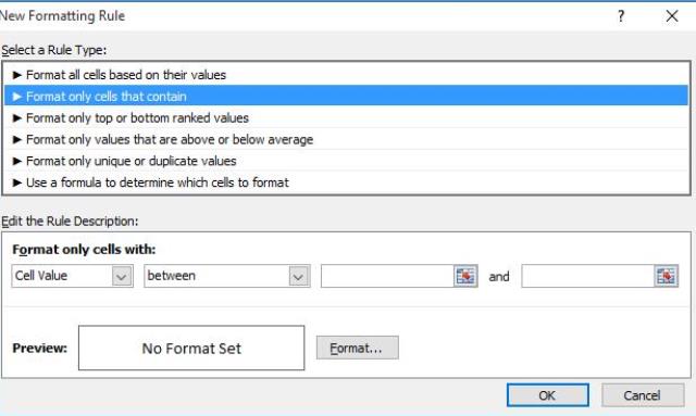
Click on “New Rules” which will open following window:-
You can see many rules in above window,
but click on “format only cells that contain”, which will extend to following
window:-
Find Eldest Student through Conditional
Formatting in Excel
To find the eldest student through
conditional formatting in excel, we can find it through only birth date
columns. So, we will apply conditional formatting on “ Birth Date” Column i.e.
Column “E”.
We will highlight here that Microsoft
Excel or any other database software considers time and dates as digit. For
instance we have write “22 Dec 20” in date formats, MS Excel will give value it
equal to 44187; or we type 5-May-05 then; excel will consider it equal to
38477. These values define that lesser value is elder date and higher value is
equal to the youngest date. Apply following method to apply to find eldest
student in school or class.
Highlight whole birthdate column i.e
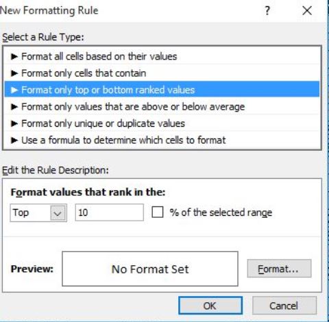
Column “E”; then click on conditional formatting from home tab. Click “New
Rule” Option which will open “New Formatting Rule” window. Click on the option
“Format only top or bottom ranked values”. This command will lead to following
window having options top or bottom. Later, select bottom option and type 1
next option button. Later click on format button shown on bottom right corner
of the window. This command will open formats window from where you can select
desired formats and then click ok. Which lead back to New Formatting rule;
where you will click OK. The eldest date will be highlighted as per desired
formats.
There are many other procedures for applying conditional formatting in MS Excel on summaries and tables of different accounts, which we shall explain in our succeeding articles.. For more details watch the video on our YouTube Channel Suhni Sindh and watch video on this link


0 Comments
Please do not enter any spam link in the comments box