COUNTIF, SUMIF Formulas and Filter Option in Excel

We have previously written about AutoSum, COUNT, COUNTA formulas. Moreover we have also demonstrated conditional formulas. Video of these formulas and conditional formulas have also been uploaded as demonstration on our YouTube Channel Suhni Sindh. We hope you must have understood. Now we are describing more functions in succeeding paragraphs.

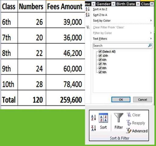
Preparation of Student Summary

We have list of all students studying in different classes but we do not know how many students are studying in each class and how much fees is being collected from each class. For analyzing these queries, we will need to prepare a summary of students showing number of students and amount being collected from them.

We can calculate all these manually but manual calculation will lead us to waste of time and chances of calculation mistakes moreover, manual summary is not feasible due to new admission and students leaving for next school or college. We are here therefore, illustrating a digitized summary of students showing each class and collection of fees.

For this purpose we shall SUMIF and COUNTIF Formulas:-

SUMIF Formula in Excel

SUMIF formula in Excel is used to calculate the figures having conditions. Suppose we have to calculate amount of fees collected from each class separately then we shall set formula to calculate fees amount separately for each class.

COUNTIF Formula in Excel

Like SUMIF Formula, COUNTIF formula in excel is used to count number of values in sheet having different conditions of the data. Follow following steps to apply SUMIF and COUNTIF formulas in Excel.

However, we shall learn to rename existing worksheet and insert new sheet in the workbook before it.  Since, apply following methods to insert and rename worksheets.

Insert Worksheet

Right click on existing worksheet name, which will show options ie. Insert, Delete, Rename, Move or Copy, View Code, Protect Sheet, Tab Color, Hide and Unhide. You may click on insert which will show what you want to insert. Select insert and click ok, which will open new sheet with the default name i.e sheet 3, sheet4 or so what.

Rename Worksheet

As mentioned above, right click on the worksheet of student data and click on rename option, which will select existing name of worksheet and rename it as Students.  Accordingly, rename newly create summary as Student Summary.

Now we shall apply COUNTIF and SUMIF Formulas as under:-

Type following columns in newly created worksheet i.e Students Summary:-

Class

Numbers

Fees Amount

Type Name of classes from 6^th to 10^th in following rows, apply formulas adjacent to each class as under and you will acquire desired values:-

Class	Numbers	Fees Amount
6th	=COUNTIF(Students!F2:F121,"6th")	=SUMIF(Students!F2:F121,"6th",Students!H2:H121)
7th	=COUNTIF(Students!F2:F121,"7th")	=SUMIF(Students!F2:F121,"7th",Students!H2:H121)
8th	=COUNTIF(Students!F2:F121,"8th")	=SUMIF(Students!F2:F121,"8th",Students!H2:H121)
9th	=COUNTIF(Students!F2:F121,"9th")	=SUMIF(Students!F2:F121,"9th",Students!H2:H121)
10th	=COUNTIF(Students!F2:F121,"10th")	=SUMIF(Students!F2:F121,"10th",Students!H2:H121)
Total	=SUM(B2:B6)	=SUM(C2:C6)

Definition of Above Formulas

COUNTIF

After starting bracket, students! Shows worksheet from where students of 6^th class are required to be counted, F2:F121 is the range of formula from where students are required be counted and “6^th” has been given criteria to the formula to count only students of sixth class,

SUMIF

Accordingly, students! Shows worksheet where students’ data is given, F2:F121, is the range of data from where students of sixth class are picked and H2:H121 is the range of amount to sum the amount collected from students.

 It is to note that the formulas we apply during our daily working on Microsoft Excel should also be analyzed manual to avoid errors at later stage. In this regards, we also can check above mentioned formula SUMIF and COUNTIF after applying filters on Students Sheet. Following is the method to check through figures through filters.

FILTER

Filter is a command or action in Microsoft Excel through which we can find values quickly. We can filter one or more columns at a time. In MS Excel 10 and latest version, we can control only one which we want to see but exclude what we want. We can create specific filters to focus the exact data.

Through FILTER we can search specific data as per our requirement through using search box of the filter interface.

How to Apply FILTER Option in Excel

Select headings row of the data or worksheet.

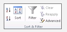
On the data tab, click on filter in the sort and filter group, which will apply filter buttons on all columns and dropdown arrow on each columns will be shown.

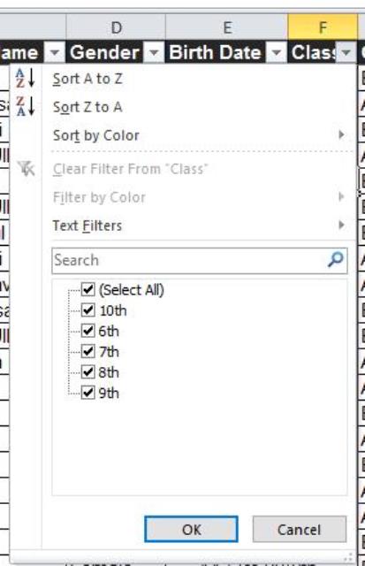
Click on dropdown arrow in the header which will display list of data which you can filter. This display will be shown depending on your data either in text, numbers or dates etc. We can filter through selecting values and can search these in search box.

We are also placing here video of COUNTIF Formula, SUMIF Formula and Applying Filter option for your easiness